DOWNLOADS


All our code is freely available for download at our Github repository
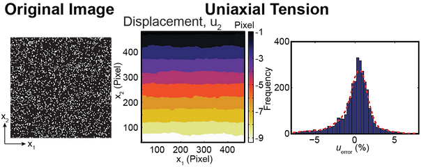
The DIC simulator is a Matlab-based GUI that assesses how “well” a particular user-provided image correlates given 4 different simulated displacement fields. The purpose of the simulator is to allow the user to optimize the speckle and intensity patterns in an image, without having to run experimentally-based calibration tests, but rather have Matlab simulate them. The DIC simulator performs the following steps:
-
User loads DIC image of interest
-
Matlab maps the intensities in the uploaded image (undeformed configuration) into a set of 4 different analytically predetermined deformation fields
-
A standard DIC algorithm correlates each image pair (deformed-undeformed config.) per given deformation field and returns the displacement matrices u1 and u2
-
The Matlab-GUI plots the determined displacement field as color contours, and as histograms of the error difference between the analytically-prescribed and DIC correlated displacement fields
The DVC simulator is the 3D cousin of the DIC Simulator. It’s also a Matlab-based GUI that assesses how “well” a particular user-provided volumetric image correlates given 4 different simulated 3D displacement fields. The import format for the 3D image stack is .mat, which is a 3x3 matrix (intensity values are stored at every x,y,z position). The purpose of the simulator is the same as for the DIC simulator, and we have found it to be of significant time and effort savings.
Health Warning
The DVC simulator requires a 3D stack to be read in, which depending on the volume size can require a large amount of RAM in Matlab, and thus when running the simulator from a laptop, we strongly suggest to use the resize option within the GUI to decrease the total stack dimensions. My macbook air can only handle 128 x 128 x 96 sufficiently.

The FIDVC algorithm is the next generation DVC algorithm providing significantly improved signal-to-noise, and large (finite) deformation (incl. large rotations and image stretches) capture capability at low computational cost (please see Bar-Kochba, Toyjanova et al., Exp. Mechanics, 2014 for more details). (File size: 751 MB) A digital image correlation version of the code is also available for download.
The following zip file contains the Matlab m-files for our FIDVC algorithm. The FIDVC algorithm is similar to our previous DVC algorithm in that it determines the 3D displacement fields between consecutive volumetric image stacks.
To provide maximum user versatility the current version is the CPU-based version, which runs a little bit slower (~ 5 - 15 minutes/per stack) than the GPU-based implementation. As Matlab’s GPU-based subroutines become more efficient we hope to provide the GPU-based version at a later release date.
To get started please open the README.txt file after download. We suggest to run the included example case first (“exampleRunFile.m” ) and compare its displacement outputs to the contour plots in the referenced paper (Bar-Kochba, Toyjanova et al., Exp. Mechanics, 2014).


This zip file contains the Matlab m-files to run our LD 3D TFM algorithm. The first part of the package includes the FIDVC algorithm, which is how the 3D displacement fields are calculated. The second part of the code package includes converting those displacement fields into 3D surface tractions as described in Toyjanova, Bar-Kochba et al., PloS One, 2014. (File size: 751 MB)
Depending on the geometry of the problem at hand, the included surface normal finder algorithm might need additional modification for traction calculation in fully embedded systems or on arbitrary geometries. Alternatively, the user can supply the his/her own point-by-point surface normals to calculate the surface tractions (e.g., Matlab has several already existing image processing options for extracting surface normals from rendered surfaces).